How electromagnetic radiation sheds light on dark clouds
Issue 110: Sept/Oct 2016
Rain, high winds, and thunderstorms can put a damper on any sailor’s day. But forewarned is forearmed, and the best resource for monitoring the locations and movement of thunderstorms is Doppler weather radar. In this first of a two-part series, Mark Thornton explains the basics of how the radar works and describes the most common types of image created from the data.
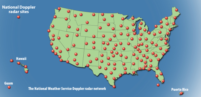
The National Weather Service’s Doppler weather radar network is comprised of 155 ground-based stations strategically placed to provide coverage over major population centers. Overlap in the system ensures continuous coverage in the event a station is offline for maintenance or due to an unplanned outage.
As a station’s antenna spins, it emits very short bursts of energy pulses (at a wavelength of 10.7 cm) that travel radially away from the station at nearly the speed of light. If these pulses encounter a target, such as a raindrop, hailstone, bird, insect, or other object, a portion of the energy is reflected back to the station — backscattered. Although it sends out pulses 1,300 times a second, the station spends the vast majority of its time listening for, and extracting data from, the backscattered energy.
A lot of useful information is derived from the pulses, such as the target’s direction and distance from the station, its height above the ground, its shape, and other physical characteristics. While the wavelength of backscattered pulses doesn’t change, the frequency of the pulses shifts based on the movement of the target. By detecting this change — the Doppler shift — the station can determine if the object is moving toward or away from the station and the speed at which it is moving.
Data from the radar can be used to create several types of imagery. The two most commonly used are reflectivity imagery and velocity imagery.
Doppler imagery: reflectivity
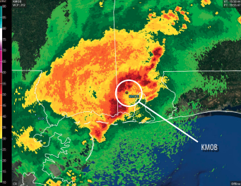
Reflectivity imagery is very useful in assessing the overall size, intensity, and evolution of a weather system. Reflectivity is the amount of energy, measured in dBZ, that is back-scattered by a target. It is related to the precipitation rate (how hard it’s raining) and varies dramatically based on the size, number, shape, and state (liquid or frozen) of targets. Values less than 20 dBZ indicate mist, dust, and other small particles. Extremely small particles, such as cloud droplets, are too small to be detected by NWS radar. Reflectivity values associated with rainfall range from 20 dBZ to 50 dBZ, depending on the number and size of the raindrops. Hail is typically present when dBZ values are greater than 55.
Reflectivity imagery is presented in two ways, base and composite. Base reflectivity displays only the data collected from the lowest layer of the atmosphere. Composite reflectivity, as the name suggests, merges the data from multiple layers of the atmosphere into a single image. By presenting more data, composite reflectivity allows for a more complete analysis of a storm system’s structure and evolution. Viewing a loop of reflectivity images is a very effective way of determining the direction a weather system is moving.
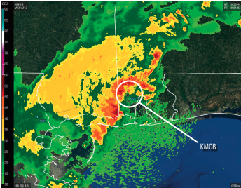
Color schemes vary based on the imagery source, but higher dBZ values are usually represented with brighter colors. On the composite reflectivity image (below), light rainfall (< 30 dBZ) is represented by shades of green. Yellow and gold show areas of moderate rainfall (30 to 40 dBZ). The most intense rainfall (and possibly hail) associated with the strongest thunderstorms appears as oranges and reds (≥ 40 dBZ). The small area of purple southwest of the station KMOB represents dBZ values greater than 60 and the presence of hail.
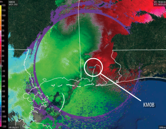
Doppler shift, velocity imagery displays the overall wind field relative to the station.
On the velocity image, the scale is in knots, with negative values indicating wind blowing toward the station (inbound) and positive values representing wind blowing away from the station (outbound). (Purple shading on velocity images indicates where the station was unable to determine the Doppler shift.) Due to the curvature of the Earth, the altitude of a radar beam steadily increases as distance from the station increases. Because of this behavior, except for areas near the station, the wind speed represented on velocity imagery is not the wind speed at the surface.
On the sample velocity image (below), the bright green shading west of the station KMOB indicates speeds of negative 30 to negative 40 knots (wind blowing toward the station) while the red shading east of the station indicates outbound winds of 20 to 40 knots. From this data, we can determine the wind is westerly. While assessing the overall wind field is useful, the true value of velocity imagery is that it enables us to monitor the speed and movement of storms. The velocity data tells us the thunderstorm cluster was approaching the station at approximately 40 knots.
Mark Thornton has been sailing on the Great Lakes for more than 20 years and currently owns Osprey, a C&C 35. His company, LakeErieWX, focuses on providing marine weather education seminars, case studies, and forecasting resources to recreational boaters. His website is www.LakeErieWX.com.
In part two of this series, in the November issue, Mark will discuss the behavior of radar beams and radar anomalies, and offer a few guidelines for using radar imagery to help visualize the dynamics and movements of weather systems.
Thank you to Sailrite Enterprises, Inc., for providing free access to back issues of Good Old Boat through intellectual property rights. Sailrite.com